Virtual Space Telescope Online

For centuries humanity has gazed upward aiming optical instruments at the night sky to unravel the mysteries of the cosmos. The evolution of observation has transitioned from rudimentary glass lenses to massive orbital observatories. Today a new paradigm has emerged in the form of the Virtual Space Telescope Online. This platform represents a sophisticated convergence of computational mathematics, rigorous astrophysics, and advanced 3D web rendering. By simulating the universe within a digital environment users are no longer bound by weather conditions, atmospheric distortion, or geographic limitations. Instead you gain unprecedented access to an interactive universe where space and time can be manipulated to understand complex astronomical phenomena.

Operating a virtual observatory is fundamentally different from simply looking at static images. The engine driving this platform processes real-time telemetry, spatial coordinates, and dynamic lighting models. When you observe Jupiter or zoom past the rings of Saturn you are interacting with mathematical algorithms calculating planetary rotations, orbital trajectories, and light scattering. This tool is designed for students, educators, and aerospace engineers who require a reliable interactive model to visualize distances that are otherwise incomprehensible to the human mind. The architecture handles everything from local planetary scales to the vast emptiness of the interstellar medium using programmatic precision.

🔭 The core philosophy behind this application is uninterrupted immersion backed by scientific accuracy. Traditional astronomy requires calculating right ascension and declination to find targets. Here the user interface abstracts these complexities while retaining the underlying physics. By manipulating the virtual focal length and field of view you emulate the optical properties of professional telescopes. The transition from a wide-angle galactic overview to a narrow-field planetary observation relies on dynamically adjusting camera matrices. This ensures that spherical bodies maintain their geometric integrity without suffering from tangential edge stretching known as perspective distortion.

The Mathematics of Planetary Motion and Orbital Mechanics

Celestial bodies do not simply float in a void; they are bound by the invisible tether of gravity. The virtual space simulation utilizes classical mechanics to position every planet, moon, and star. To achieve realistic representations the engine relies on the principles established by Kepler and Newton. The movement of an object in a stable orbit requires a delicate balance between its forward velocity and the gravitational pull of its parent body. While the virtual telescope allows you to instantly traverse these distances the spatial relationships are modeled on exact proportions.

One of the foundational calculations in astrophysics is determining the orbital period of a celestial body. According to Kepler’s Third Law the square of the orbital period is proportional to the cube of the semi-major axis of its orbit. In a simulated environment this dictates how fast a planet must travel along its path. The simplified mathematical representation is formulated as

T² = a³

where T represents the time in Earth years and a represents the distance in Astronomical Units. When calculating exact physical forces Newton’s law of universal gravitation is applied. The force between two masses is determined by

F = G * M₁ * M₂ / r²

In this equation G is the gravitational constant, M variables denote the mass of the respective bodies, and r is the distance between their centers.

To accurately render a spacecraft or a satellite entering orbit the concept of orbital velocity is crucial. The speed required to maintain a stable circular orbit near a planet is calculated using

v = √GM / r

If an object needs to break free from the gravitational influence entirely it must reach escape velocity. This requires significantly more energy and is represented by the formula

v_e = √2GM / r

The virtual engine uses variations of these formulas to plot accurate trajectories and ensure that objects in the simulation behave according to the laws of physics. Understanding these parameters is essential for aerospace engineering and planning deep space missions.

Celestial Body	Distance from Sun AU	Orbital Period Years	Base Equatorial Radius km
Mercury	0.39	0.24	2440
Venus	0.72	0.62	6051
Earth	1.00	1.00	6371
Mars	1.52	1.88	3389
Jupiter	5.20	11.86	69911
Saturn	9.58	29.46	58232
Uranus	19.20	84.01	25362
Neptune	30.05	164.80	24622

Optical Emulation and Virtual Magnification Parameters

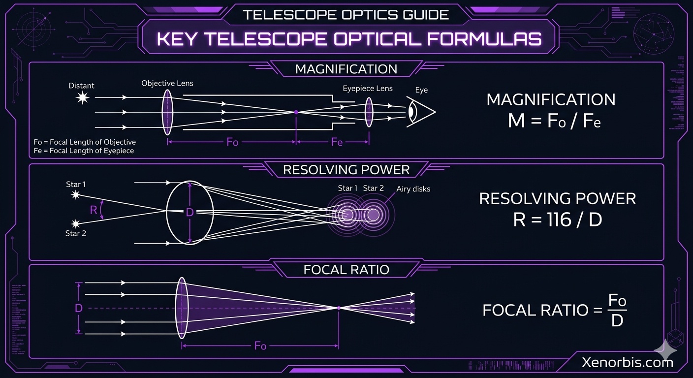
The true power of the Virtual Space Telescope lies in its ability to mimic physical optics through digital rendering. In terrestrial astronomy an observer changes eyepieces to alter the magnification and field of view. The digital counterpart achieves this by manipulating the camera projection matrix. By lowering the field of view angle the application artificially lengthens the focal length creating a powerful zoom effect. This technique eliminates the spherical aberrations and chromatic distortions that plague physical glass lenses allowing for crystal clear observations of distant orbital bodies.

To calculate the magnification power of a real telescope astronomers use a straightforward relationship. The magnification is equal to the focal length of the objective lens divided by the focal length of the eyepiece. Written out this is

M = F_o / F_e

When utilizing the online simulator the zoom slider mathematically adjusts the virtual camera coordinates mimicking this exact optical transition. Furthermore the resolving power which dictates the smallest detail a telescope can distinguish is dependent on the diameter of its primary mirror. The Dawes limit states that the resolving power in arcseconds is

R = 116 / D

where D is the aperture in millimeters. In our digital universe the rendering resolution is limited only by the pixel density of the user’s monitor and the quality of the texture mapping.

Lighting is another critical component in simulating space. The sun acts as a point light source radiating energy outward. As light travels through space its intensity diminishes based on the inverse square law. The apparent brightness of a celestial object is determined by its luminosity and its distance from the observer. The equation is

E = L / 4πd²

where E is the observed flux, L is absolute luminosity, and d is the distance. The rendering engine utilizes High Dynamic Range tone mapping specifically Reinhard algorithms to manage these extreme contrasts. This ensures that the glaring brilliance of a star does not completely wash out the subtle details of nearby planetary surfaces or nebula gas clouds.

Optical Concept	Equation Formula	Primary Variable	Practical Application
Magnification	M = Fo / Fe	Focal Lengths	Determines target size in eyepiece
Focal Ratio	f-ratio = Fo / D	Aperture D	Calculates photographic speed
Resolving Power	R = 116 / D	Objective Diameter	Defines maximum image sharpness
Light Gathering	LGP = D2 / de2	Eye Pupil de	Measures brightness relative to human eye

Traversing Deep Space Galaxies and Nebulae

Beyond the borders of the local solar system the scale of the universe changes drastically. Measuring distance in kilometers or even Astronomical Units becomes highly impractical. Astronomers switch to lightyears and parsecs. To bridge this conceptual gap the Virtual Space Telescope incorporates a logarithmic depth system. When you zoom outward past the orbit of Neptune the spatial engine smoothly transitions its scale. This prevents floating point precision errors a common issue in 3D rendering where objects far from the origin begin to jitter. By resetting the relative focal point the observer can seamlessly travel from a tight orbit around the Moon to the outer edges of distant galaxy clusters.

Nebulae are rendered using additive blending techniques. Unlike solid geometric shapes clouds of interstellar gas do not block light; they accumulate it. By layering multiple translucent particle textures with varying hues the system emulates the emission of ionized gases. Stellar classification plays a major role in determining the color of the stars populating these fields. The surface temperature of a star dictates its exact spectral signature ranging from cool red dwarfs to blistering blue giants.

Spectral Class	Temperature Kelvin	Visual Color	Main Sequence Example
O Class	Over 30,000 K	Blue	Zeta Puppis
B Class	10,000 to 30,000 K	Blue White	Rigel
A Class	7,500 to 10,000 K	White	Sirius
G Class	5,200 to 6,000 K	Yellow	The Sun
M Class	Under 3,700 K	Red	Proxima Centauri

Advanced Visualization Techniques for Web Applications

Building a high performance virtual observatory in a web browser requires overcoming significant technical hurdles. The application must render high resolution textures up to 8K in quality mapped onto dense spherical geometries without dropping frame rates. This is achieved through aggressive resource management. The planets are not merely painted spheres; they utilize complex shader materials. Earth for instance features a basic color map layered with a specular map to distinguish the reflective properties of oceans from the matte finish of landmasses. An additional atmospheric layer is generated slightly larger than the planet mesh to simulate Rayleigh scattering causing the blue halo effect seen from orbit.

🪐 For celestial bodies with ring systems like Saturn the geometry becomes more intricate. Rings are not solid objects but massive collections of ice and rock dust. The virtual telescope replicates this using flat ring geometries equipped with double sided materials and transparency maps. This allows the observer to view the rings from any angle whether illuminated from above or casting shadows from below. The tilt of these rings which significantly impacts their visibility from Earth is strictly adhered to in the coordinate mapping process.

Space debris and artificial satellite tracking represent another layer of complexity. The orbital space immediately surrounding Earth is highly congested. Tracking these objects requires processing Two Line Element data sets which provide the precise orbital parameters of every documented object. Calculating the position of a satellite involves determining its eccentric anomaly. Kepler’s equation must be solved iteratively because it cannot be rearranged to solve for E directly. The 3D engine computes this in real time allowing users to visualize the expanding cloud of space debris tracking individual orbits and calculating potential conjunctions based on exact physical trajectories.

The Future of Digital Stargazing and Education

The accessibility provided by the Virtual Space Telescope Online bridges the gap between passive observation and active scientific inquiry. Users are empowered to conduct independent experiments regarding planetary alignment tracking historical eclipses and understanding the vast scale of the universe. By adjusting the field of view rendering limits and exposure settings you gain practical experience in the mechanics of astrophotography without the need for expensive hardware.

Furthermore the underlying architecture is highly modular allowing for continuous integration of new astronomical data. As real world space agencies discover new exoplanets or capture high definition mapping of distant asteroids this information can be parsed into the simulation. The rendering engine’s ability to handle procedural generation means that the entire known universe can be mapped and visualized dynamically. The optimization of buffer geometries ensures that even modest computational devices can handle the processing required to display tens of thousands of stars simultaneously.

For those interested in the rigorous engineering behind such tools mastering the combination of orbital mathematics and 3D web programming is essential. The formulas provided here serve as the baseline for translating physical reality into digital environments. Whether you are calculating the precise amount of fuel required to shift an orbit using the Tsiolkovsky rocket or programming a complex planetary gear mechanism for a tracking mount the intersection of coding and astronomy offers endless possibilities for innovation.

Recommended Reading for Space Engineering and Astronomy

• Orbital Mechanics for Engineering Students by Howard D. Curtis — A comprehensive mathematical breakdown of satellite motion trajectory planning and celestial mechanics.
• Fundamentals of Astrodynamics by Roger R. Bate — An absolute classic providing the core formulas and concepts required for understanding space flight and planetary orbits.
• Astronomy: A Physical Perspective by Marc L. Kutner — Connects the visual observations of the night sky with the underlying physics and mathematical laws governing the universe.
• The Dobsonian Telescope: A Practical Manual for Building Large Aperture Telescopes by David Kriege — Essential reading for understanding telescope optics focal ratios and physical observatory engineering.
• Real-Time Rendering by Tomas Akenine-Möller — The definitive guide to the mathematics and programming techniques behind advanced 3D graphics shading and lighting models.