
Orbital mechanics sounds intimidating. It immediately evokes images of chalkboards covered in abstract Greek symbols and complex equations. Yet, when visualized live, the chaotic choreography of spaceflight resolves into beautiful, logical geometric patterns. Human beings have maintained a continuous presence in Low Earth Orbit for decades, relying on a delicate balance of speed, altitude, and gravity to keep multi-billion dollar research facilities from plummeting back to the surface. This reference guide bridges the gap between raw astrodynamics and the visual feedback provided by modern tracking tools, turning an invisible celestial highway into a tangible grid for enthusiasts and developers alike.
🛰 To truly appreciate what happens inside a digital simulation environment, one must discard terrestrial biases. On the ground, moving forward requires continuous propulsion to overcome friction. In the vacuum of space, movement is governed by inertia and the curvature of space-time. Understanding how a space station sustains its flight path is the first step toward mastering the variables found within tracking software and interactive engines.
Contents
The Perpetual Fall: Demystifying Weightlessness
Gravity never actually stops in space. A common misconception suggests that astronauts float because they are entirely clear of Earth’s gravitational pull. In reality, gravity at the average altitude of human spaceflight remains at roughly ninety percent of its surface strength. The sensation of weightlessness occurs because the vehicle and its crew are in a state of perpetual freefall toward the planet, but they possess enough forward velocity to constantly miss the horizon. As the station drops down, the surface of the globe curves away at the exact same rate.
This horizontal velocity must be precisely calculated and maintained. If the vehicle slows down by even a small fraction, its trajectory bends inward, leading to a catastrophic atmospheric reentry. Conversely, if the velocity increases beyond a specific threshold, the orbit stretches into an ellipse, pushing the craft further into deep space. The circular path utilized by most modern outposts is a highly specific sweet spot where speed matches the local pull of gravity perfectly.
The Vis-Viva Equation and Velocity Vector Relationships
To plot any spacecraft path or program its movement within a canvas container, engineers rely on foundational physics. The velocity of a satellite at any given point along its trajectory can be derived using the classical vis-viva equation, which is expressed as follows:
v2 = G × M × (2 / r – 1 / a)
Within this relationship, v represents the orbital velocity of the spacecraft. The product of G, the universal gravitational constant, and M, the mass of the parent planet, is known as the standard gravitational parameter. The variable r dictates the current radial distance from the center of the world to the object, while a represents the semi-major axis of the entire trajectory. For a perfectly circular flight path, the semi-major axis equals the radial distance, simplifying the math down to a direct calculation of constant circular speed.
v = (G × M / r)0.5
This fundamental speed requirement means that closer outposts must fly significantly faster than those located further away from the planet. A station orbiting just a few hundred kilometers up clocks speeds that allow it to circle the entire globe in roughly ninety minutes, a blistering pace that poses unique challenges for visual rendering and tracking algorithms.
The Keplerian Elements: Six Coordinates of Freedom
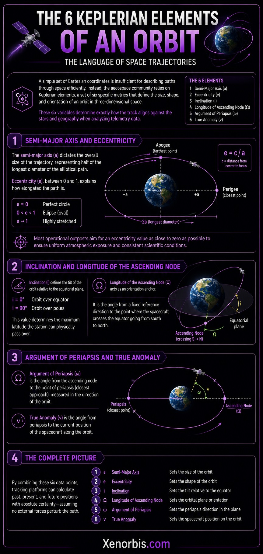
A simple set of Cartesian coordinates is insufficient for describing paths through space efficiently. Instead, the aerospace community relies on Keplerian elements, a set of six specific metrics that define the size, shape, and orientation of an orbit in three-dimensional space. When analyzing telemetry data within a visualization tool, these six variables determine exactly how the track aligns against the stars and geography.
Semi-Major Axis and Eccentricity
The semi-major axis dictates the overall size of the trajectory, representing half of the longest diameter of the elliptical path. It establishes the baseline energy of the spacecraft. Eccentricity, denoted as a value between zero and one, explains how elongated the path is. A value of zero represents a perfect circle, while values approaching one indicate highly stretched ovals. Most operational scientific outposts aim for an eccentricity value as close to zero as possible to ensure uniform atmospheric exposure and consistent scientific testing conditions.
Inclination and Longitude of the Ascending Node
Inclination defines the tilt of the flight path relative to the equatorial plane of the planet. An inclination of zero degrees means the station flies directly above the equator, whereas a ninety-degree inclination sends the craft directly over the North and South poles. This value determines the maximum latitude the station can physically pass over during its mission. The Longitude of the Ascending Node acts as an orientation anchor, mapping the exact point where the spacecraft crosses the equator while traveling from the southern hemisphere to the northern hemisphere.
Argument of Periapsis and True Anomaly
The argument of periapsis serves as the internal orientation angle of the ellipse, pointing out where the closest approach to the planet occurs along the orbital ring. Finally, the True Anomaly defines the actual location of the physical spacecraft along that established path at a specific moment in time. By combining these six data points, tracking platforms can calculate past, present, and future positions with absolute certainty, assuming no external forces perturb the path.
Historical and Contemporary Space Station Parameters
Humanity has launched multiple modular habitats into the upper reaches of the atmosphere since the mid-twentieth century. Each project requires a unique orbital configuration based on its launch site, mission goals, and international partnerships. Comparing these designs reveals how political and physical constraints shape the layout of our cosmic infrastructure.
| Spacecraft Name | Average Operational Altitude | Orbital Inclination Angle |
|---|---|---|
| International Space Station | 420 Kilometers | 51.64 Degrees |
| Tiangong Space Station | 390 Kilometers | 41.58 Degrees |
| Mir Orbital Complex | 360 Kilometers | 51.60 Degrees |
| Skylab Laboratory | 435 Kilometers | 50.00 Degrees |
| Salyut 7 Research Station | 219 Kilometers | 51.60 Degrees |
The specific inclination of fifty-one point sixty-four degrees used by the International Space Station was not selected at random. It was a carefully negotiated compromise allowing launch vehicles departing from both Baikonur in Kazakhstan and Cape Canaveral in Florida to safely reach the complex without flying over heavily populated areas or violating foreign airspace during stage separation.
Atmospheric Layers and Environmental Degradation
Space does not begin abruptly at a crisp line, despite arbitrary legal definitions like the Kármán line. The gas surrounding our planet thins out exponentially, meaning that platforms flying at altitudes between three hundred and six hundred kilometers are still interacting with the outermost wisps of the atmosphere, specifically the thermosphere and exosphere. This interaction introduces real-world mechanics that interactive programs must account for over long timelines.
| Altitude Threshold | Dominant Atmospheric Particle | Primary Vehicle Impact |
|---|---|---|
| 100 to 200 Kilometers | Molecular Nitrogen | Extreme aerodynamic drag and rapid decay |
| 200 to 400 Kilometers | Atomic Oxygen | Material erosion and measurable deceleration |
| 400 to 700 Kilometers | Helium Atoms | Minor drag variations based on solar cycles |
| Above 700 Kilometers | Hydrogen Ions | Negligible gas interactions, radiation dominance |
Atomic oxygen presents a dual threat to low-flying hardware. Formed when solar radiation breaks down standard oxygen molecules, these highly reactive single atoms constantly collide with the forward-facing surfaces of the station. This process leads to the chemical erosion of protective thermal blankets and solar panel substrates, changing their optical and structural properties over years of exposure.
The Physics of Orbital Decay and Reboost Procedures
🚀 Because gas particles exist in Low Earth Orbit, a spacecraft is constantly subject to microscopic friction. This phenomenon is known as aerodynamic drag. As the station collides with these stray atoms, it surrenders a portion of its kinetic energy. Referring back to the vis-viva equation, a loss of energy forces a reduction in the semi-major axis, causing the vehicle to slowly spiral downward toward the denser layers of air.
The rate of this decay is highly volatile and depends heavily on the activity of the Sun. During periods of solar maxima, extreme ultraviolet radiation heats the upper atmosphere, causing the thermosphere to expand outward like a warming balloon. This expansion increases the particle density at operational flight altitudes, accelerating orbital decay rates by up to a factor of ten. To counteract this relentless pull, stations must periodically fire their onboard thrusters or utilize the engines of docked cargo vehicles to perform orbital reboosts, artificially pumping kinetic energy back into the system to restore their target altitude.
Calculating Atmospheric Drag Acceleration
The deceleration force acting upon a spacecraft hull due to drag can be modeled mathematically using standard fluid dynamics, modified for hyper-rarefied gas environments. The acceleration due to drag is expressed through the following equation:
ad = 0.5 × ρ × v2 × Cd × A / m
In this scenario, ad represents the resulting deceleration vector. The variable ρ defines the local atmospheric density, which fluctuates based on altitude and solar weather. The velocity relative to the atmosphere is marked by v, while Cd is the drag coefficient of the vehicle, typically determined by its geometric profile. The variable A stands for the cross-sectional area facing directly into the velocity vector, and m represents the total mass of the station. The ratio of surface area to mass is a critical metric for orbital longevity, large solar arrays increase drag dramatically, demanding more frequent fuel expenditures to stay aloft.
Visualizing Ground Tracks and Spatial Distortion
When translating a three-dimensional path onto a two-dimensional map, tracking applications use ground tracks. A ground track is the projection of the satellite’s orbital path directly onto the surface of the Earth. Because the planet rotates beneath the spacecraft while the flight path remains fixed in inertial space, the resulting ground track forms a repeating, sinusoidal wave pattern that shifts westward with every completed revolution.
This westward shift is an illusion caused entirely by the Earth spinning on its axis at approximately fifteen degrees per hour. If a station takes ninety minutes to complete an orbit, the planet moves twenty-two point five degrees eastward during that exact window. Consequently, when the station returns to the same latitude on its next lap, it finds itself tracking over entirely new terrain located further to the west. This shifting geometry ensures that earth-observation platforms can eventually photograph almost the entire globe over a set period of days.
Astrodynamic Constants for Local System Architecture
To accurately compute coordinates, velocities, and periods inside any physical simulation script, precise mathematical values must be hardcoded into the core engine logic. Small rounding errors at the scale of planetary tracking can compound into thousands of kilometers of positional drift within a few simulated days.
| Astrodynamic Metric | Accepted Standard Value | Physical Measurement Unit |
|---|---|---|
| Geocentric Gravitational Parameter | 398600.44 | km3 / s2 |
| Mean Volumetric Earth Radius | 6371.00 | Kilometers |
| Equatorial Earth Rotation Speed | 465.10 | Meters per Second |
| Sidereal Rotation Period | 86164.10 | Seconds |
| Standard Solar Radiation Pressure | 4.56 × 10⁻⁶ | Newtons per Meter2 |
Notice that the sidereal day is slightly shorter than the standard twenty-four hour solar day. This discrepancy occurs because the Earth is also moving along its path around the Sun, meaning it must rotate slightly more than three hundred and sixty degrees relative to distant stars to bring the Sun back to the exact same spot in the sky. Precision simulators always track time using sidereal calculations to keep star maps and satellite positions perfectly synced.
Perturbations: The Realities of Non-Spherical Worlds
In elementary physics classes, planets are treated as perfect, uniform spheres. In reality, the Earth is an oblate spheroid, flattened at the poles and bulging at the equator due to centrifugal forces generated by its rotation. This asymmetric distribution of mass creates an uneven gravitational field that warps passing orbits over time. This effect is known as the J2 perturbation.
The equatorial bulge exerts a constant torque on tilted trajectories, causing two primary forms of orbital drift: nodal precession and the rotation of the apsides. Nodal precession forces the entire orbital plane to twist slowly around the rotational axis of the Earth, changing its orientation relative to the stars. Engineers can actually weaponize this perturbation to create Sun-synchronous tracks, balancing the tilt of the orbit so that it precesses at exactly the same rate the Earth circles the Sun, ensuring the satellite passes over ground points at identical local solar times every single day.
Telemetry Ingestion and Two-Line Element Sets
Real-time visualizers do not guess where space assets are located. They ingest standardized data packets generated by radar tracking networks managed by military and scientific coalitions. The most ubiquitous format for this data is the Two-Line Element set, commonly abbreviated as TLE.
A TLE is a text block containing two lines of seventy characters each, packed with encoded numerical fields. These lines define the exact Keplerian parameters of an object at a specific reference timestamp, known as the epoch. Because external variables like atmospheric drag and gravitational anomalies constantly modify actual flight paths, TLE data degrades rapidly. Tracking applications must update these text blocks every few days to maintain precision, feeding the fresh parameters into numerical propagation models like SGP4 to compute clean coordinates for rendering pipelines.
The Crucial Role of Multi-Core Time Synchronization
When running a high-speed orbital environment inside a web browser or desktop container, developers run into problems coordinating simulation time with rendering loops. If the update logic is tied directly to the graphical frame rate, variations in computing performance will cause the space station to skip erratically across the screen or fall out of alignment with the rotating globe beneath it.
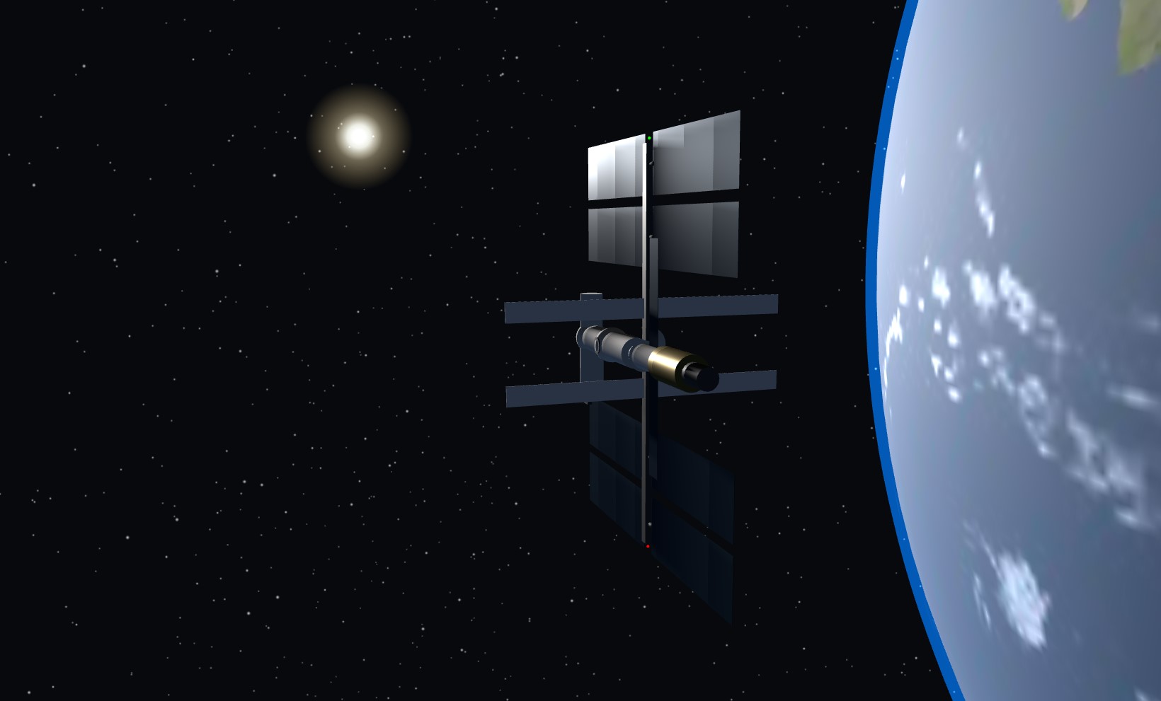
Modern engines solve this by uncoupling the physics step from the rendering cycle. The position of the spacecraft is calculated using delta time increments derived from the system clock, allowing the mathematics of the orbit to advance smoothly regardless of whether the graphics hardware is churning out thirty or one hundred and twenty frames per second. This temporal isolation is vital when running high-speed accelerations where hours of orbital flight are compressed into seconds of user interface playback.
Essential References for Astrodynamics and Flight Simulation
For individuals seeking a deeper, uncompromised technical command of orbital mechanics, spacecraft telemetry, and the physics of human spaceflight, the following literature represents the gold standard of reference texts:
- Fundamentals of Astrodynamics – Roger R. Bate, Donald D. Mueller, Jerry E. White
- Orbital Mechanics for Engineering Students – Howard D. Curtis
- Spacecraft Systems Engineering – Peter Fortescue, John Stark, Graham Swinerd
- Satellite Technology: Principles and Applications – Anil K. Maini, Varsha Agrawal
- Introduction to Space Dynamics – William Tyrrell Thomson

Julian D. Thorne — Celestial Mechanics Developer
Researcher and 3D engine developer focused on interactive stellar systems. Julian bridges the gap between theoretical physics and real-time browser-based cosmos exploration.


