Celestial mechanics has fascinated humanity for millennia, guiding ancient calendars, maritime navigation, and modern aerospace missions. Visualizing these complex three-dimensional interactions requires precise computational tools. A modern three-dimensional simulator bridges the gap between abstract gravitational formulas and intuitive visual comprehension. By modeling the spatial orientations of the Sun, Earth, and Moon, such software allows researchers, educators, and hobbyists to look into the past and predict future astronomical events with pinpoint accuracy.
🌘 Understanding these phenomena requires moving beyond two-dimensional diagrams. The cosmos operates in a continuous state of motion dictated by gravitational forces, orbital inclinations, and specific geometric alignments. This reference text breaks down the core scientific principles, mathematical foundations, and real-world applications of lunar tracking and eclipse prediction systems.
Contents
Practical Applications of Lunar and Eclipse Simulations
- Simulating the lunar cycle and orbital intersections is far more than an academic exercise. Precise predictive models are indispensable across various modern industries and scientific disciplines. Aerospace engineers rely on exact lunar coordinates to calculate trajectories for deep-space missions, lunar landers, and satellite placement. Because the Moon acts as a major source of gravitational perturbation for low Earth orbit satellites, tracking its position is essential for maintaining orbital stability and planning station-keeping maneuvers.
- In the realm of marine science, tidal forecasting relies heavily on the relative positions of the Sun and Moon. The gravitational pull of both bodies generates tidal bulges. When they align during a new or full moon, they create spring tides, which are exceptionally high. Conversely, when they sit at right angles during quarter phases, they produce weaker neap tides. Accurate simulations allow port authorities and shipping companies to predict navigable water depths months in advance.
- For observational astronomers and astrophotographers, a simulator functions as an indispensable planning tool. Capturing a total solar eclipse or a subtle penumbral lunar eclipse requires knowing the exact second of contact, the path of totality, and local atmospheric conditions. Software allows photographers to pre-visualize the field of view, calculate the required focal length, and optimize exposure times based on the projected illumination of the lunar surface.
- Historians and archaeologists also utilize these systems to date ancient events. Many ancient texts describe unexpected daytime darkness or unusual full moons during major battles or reigns of monarchs. By running orbital simulations backward through time, researchers can pinpoint the exact day and year these historical events occurred, providing an absolute chronological anchor for historical research.
Decoding the Lunar Cycle: Synodic versus Sidereal Periods
To build an accurate simulator, one must separate the two distinct ways of measuring a lunar month. The difference arises because the Earth is constantly moving along its own orbit around the Sun while the Moon orbits the Earth. This dual orbital motion introduces a shift in perspective that alters the time required to complete a cycle of phases versus a true 360-degree orbit.
The sidereal month represents the true orbital period of the Moon relative to the distant, fixed stars. It is the time required for the Moon to return to the exact same position on the celestial sphere. This orbital journey takes approximately 27.32166 days. If the Earth stood completely still, the cycle of lunar phases would match this number exactly.
🌗 However, because the Earth advances along its elliptical path around the Sun by about one degree per day, the Moon must travel a bit further to return to the same spatial alignment relative to the Sun and Earth. This phase-to-phase cycle is known as the synodic month, or lunation. Spanning roughly 29.53059 days, the synodic month dictates the familiar progression from new moon to full moon and back again. The interactive software incorporates this continuous orbital shifting to display the correct illumination percentage for any selected calendar date.
During this synodic period, the visible portion of the Moon changes systematically. This progression is divided into eight primary phases, determined by the elongation angle between the Moon and the Sun as viewed from Earth. When the Moon sits directly between the Earth and the Sun, its illuminated side faces away from us, resulting in a new moon. As it moves eastward along its orbit, the crescent grows, passes through the first quarter at a 90-degree alignment, becomes gibbous, and reaches full moon status when it stands opposite the Sun at an angle of 180 degrees. The reverse process occurs during the waning half of the cycle.
The Reference Guide to Lunar Phase Characteristics
The following dataset details the specific attributes of the primary and intermediate lunar phases as tracked by modern computational models. This data assumes an average synodic month and standard orbital velocity.
| Phase Name | Average Age in Days | Illumination Range | Position Relative to Sun |
|---|---|---|---|
| New Moon | 0.0 to 1.0 | 0% | Conjunction at 0 degrees |
| Waxing Crescent | 1.1 to 6.4 | 1% to 49% | Western sky after sunset |
| First Quarter | 6.5 to 8.4 | 50% | Quadrate at 90 degrees |
| Waxing Gibbous | 8.5 to 13.7 | 51% to 99% | High in sky at dusk |
| Full Moon | 13.8 to 15.8 | 100% | Opposition at 180 degrees |
| Waning Gibbous | 15.9 to 21.1 | 99% to 51% | High in sky at dawn |
| Third Quarter | 21.2 to 23.1 | 50% | Quadrate at 270 degrees |
| Waning Crescent | 23.2 to 28.5 | 49% to 1% | Eastern sky before sunrise |
The Three-Dimensional Geometry of Eclipses
If the Moon’s orbit sat in the exact same plane as the Earth’s orbit around the Sun, an eclipse would occur twice every single month. We would witness a solar eclipse at every new moon and a lunar eclipse at every full moon. In reality, these spectacles are relatively rare occurrences due to a crucial structural tilt in the lunar path.
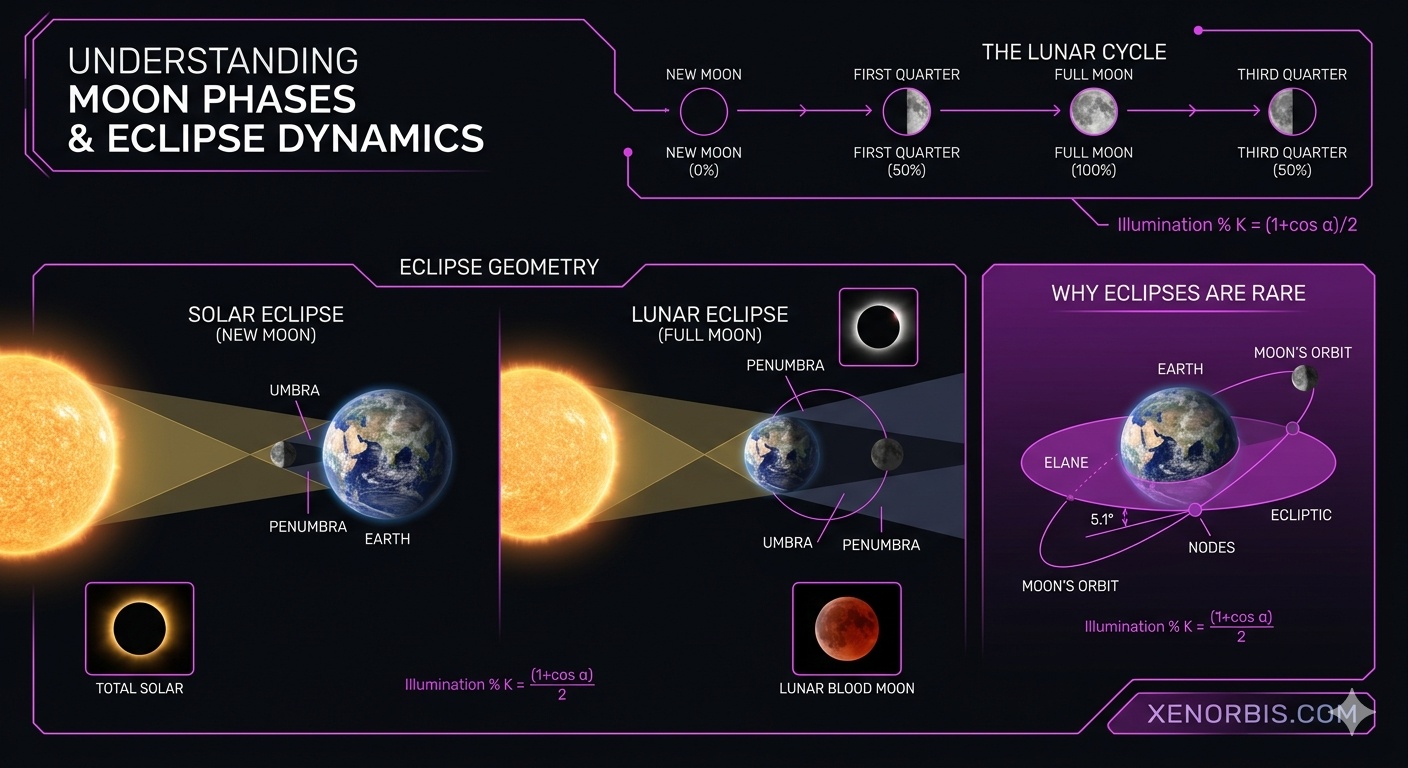
The orbit of the Moon is inclined by approximately 5.14 degrees relative to the ecliptic plane, which is the plane of Earth’s orbit around the Sun. Because of this inclination, the Moon spends most of its time either above or below the direct line connecting the Earth and the Sun. Its shadow usually misses the Earth entirely during a new moon, passing harmlessly out into empty space, while the Earth’s shadow misses the Moon during a full moon.
For an eclipse to take place, two conditions must be met simultaneously. First, the Moon must be in the correct phase, either new for a solar eclipse or full for a lunar eclipse. Second, the Moon must be positioned at or very close to one of the two points where its tilted orbit intersects the ecliptic plane. These intersection points are called the orbital nodes. The straight line connecting these two points is known as the line of nodes.
When the line of nodes aligns directly with the Sun during a new or full moon, a alignment known as syzygy occurs. This alignment opens up a brief window of opportunity called an eclipse season. Because the line of nodes slowly drifts over time due to the gravitational tug of the Sun, the timing of these seasons shifts backward through the calendar year, completing a full revolutionary cycle every 18.6 years.
Classifying Eclipse Typologies and Structural Variations
Eclipses vary dramatically in appearance and duration depending on the precise distances and spatial alignments of the three celestial bodies. The following reference matrix categorizes these events based on their geometric properties.
| Eclipse Typology | Required Phase | Node Proximity Constraint | Visual Manifestation |
|---|---|---|---|
| Total Solar | New Moon | Extremely Close [Under 4.5 degrees] | Sun completely blocked by Moon |
| Annular Solar | New Moon | Close [Moon near apogee] | Ring of fire around lunar silhouette |
| Partial Solar | New Moon | Moderate [Edge of eclipse window] | Sun appears partially bitten |
| Total Lunar | Full Moon | Extremely Close [Under 3.8 degrees] | Moon turns deep copper red |
| Partial Lunar | Full Moon | Moderate [Partial umbral entry] | Earth shadow darkens a fraction |
| Penumbral Lunar | Full Moon | Distant [Misses core umbral shadow] | Subtle, dimming of lunar brightness |
Mathematical Foundations of Celestial Tracking
To convert visual descriptions into functional code, simulators implement fundamental equations derived from Newtonian physics and Keplerian orbital mechanics. These mathematical formulas dictate how the virtual camera, light sources, and spheres interact over time.
The relationship between the synodic period and the sidereal periods of the Earth and Moon can be expressed through a simple harmonic frequency equation. If Tsyn represents the synodic month, Tsid represents the Moon’s sidereal orbital period, and Tearth represents the Earth’s sidereal orbital period around the Sun, the formula is structured as follows:
1 / Tsyn = 1 / Tsid – 1 / Tearth
By solving for Tsyn, software engineers can program the precise rate at which the light source changes angle relative to the virtual camera, ensuring the phasing animation remains synchronized over long simulation runs.
To calculate the exact illumination fraction of the lunar disc visible from Earth, the system must determine the phase angle. Let α be the topocentric elongation angle between the Sun and the Moon as observed from the center of the Earth. The fraction of the visible disk that is illuminated, denoted as k, is calculated using the following trigonometric relationship:
k = [1 + cos α] / 2
When α equals 0 degrees, the cosine is 1, yielding k = 1, which represents a completely illuminated full moon. At a 90-degree angle, the cosine becomes 0, resulting in k = 0.5, or a half-illuminated quarter moon. When the angle reaches 180 degrees, the cosine is -1, giving k = 0, which corresponds to a completely dark new moon.
The speed of the Moon as it moves along its elliptical path is not constant. It accelerates when it draws closer to the Earth at perigee and decelerates when it moves further away at apogee. To model this variable motion, simulators utilize the Vis-Viva equation, which is derived from the conservation of orbital energy. Let v be the instantaneous relative velocity, G be the universal gravitational constant, M be the mass of the Earth, r be the current distance between the two bodies, and a be the semi-major axis of the orbit:
v2 = G × M × [2 / r – 1 / a]
This velocity variance directly affects the exact timing of eclipses. It also influences a phenomenon known as lunar libration, which causes the Moon to appear to nod slightly back and forth, allowing observers on Earth to see roughly 59% of its surface over time.
To determine the orbital size and time parameters, Kepler’s Third Law provides a foundational mathematical link. The square of the orbital period T is directly proportional to the cube of the semi-major axis a. When accounting for the masses of both the Earth, denoted as M, and the Moon, denoted as m, the formula reads:
T2 = [4 × π2 / [G × [M + m]]] × a3
Using this law, if a simulation alters the distance parameter between the bodies to demonstrate alternative physical scenarios, it can automatically scale the time factor to keep the system physically consistent.
Finally, predicting the recurrence of eclipses over centuries involves tracking the Saros cycle. This specific interval spans exactly 223 synodic months, which correlates with three separate lunar orbital cycles: the synodic month, the draconic month, and the anomalistic month. The mathematical identity that defines this cyclical harmony is expressed as:
223 × Tsyn ≈ 242 × Tdrac ≈ 239 × Tanom
This product amounts to approximately 6585.3211 days, or 18 years, 11 days, and 8 hours. Because of the extra eight-hour fraction, the Earth rotates an additional one-third of a turn before the next eclipse in the series occurs, shifting the path of totality 120 degrees westward on the globe. Modern simulators use this relationship to group related eclipse events into long historical series.
Advanced Orbital Parameters and System Constraints
☀ High-fidelity simulations must account for subtle gravitational anomalies caused by external factors. The simple two-body problem assumes perfectly spherical masses operating in a total vacuum. In our actual solar system, the immense gravitational field of the Sun continuously distorts the lunar orbit, pulling it out of a perfect ellipse.
The key values required to configure a highly accurate simulation environment are compiled in the reference table below. These metrics represent the standard baseline figures used in modern astronomical tracking systems.
| Orbital Parameter | Standard Baseline Value | Time Period of Variation | Impact on Simulation Architecture |
|---|---|---|---|
| Semi-major Axis | 384,400 kilometers | Constant average | Sets the master scale of the rendering canvas |
| Orbital Eccentricity | 0.0549 | Periodic fluctuation | Controls the elliptical stretching of the path |
| Nodal Precession Period | 18.61 Julian years | Continuous retrograde | Rotates the 3D orbit plane around the ecliptic axis |
| Apsidal Precession Period | 8.85 Julian years | Continuous prograde | Rotates the major axis orientation over time |
The nodal precession listed above is particularly vital for long-term tracking. Because the orbital nodes slide backward along the ecliptic plane, the spatial location where eclipses can occur is constantly moving. A simulator that fails to implement this 18.6-year rotational cycle will produce cumulative errors, leading to completely incorrect eclipse predictions within just a few simulated calendar years.

Another major factor is the tilt of the Earth’s own rotational axis, which sits at roughly 23.44 degrees relative to the ecliptic plane. This tilt creates our terrestrial seasons. It also changes the apparent path of the Moon across the night sky depending on the observer’s latitude. When combined with the 5.14-degree lunar inclination, the maximum altitude of the Moon above the horizon can vary by nearly 10 degrees over the course of the broader nodal cycle. This variation creates periods known as major and minor lunar standstills.
How Engine Software Replicates Lunar Kinematics
To convert these mathematical principles into a real-time interactive experience, software developers utilize specialized rendering strategies. The system tracks time using Julian Dates, a continuous count of days since a standardized historical epoch. This approach avoids the computational complexities of standard calendar months and leap years. By feeding the Julian Date into positional algorithms, the software computes the precise 3D vector coordinates for the Sun, Earth, and Moon.
Once the coordinates are calculated, a graphic engine draws the objects inside a virtual space. The rendering engine applies directional light sources from the Sun’s coordinate vector toward the Earth and Moon models. To make the phases look realistic, the software applies advanced shading calculations. While a standard smooth plastic sphere reflects light evenly, the real Moon is covered in highly textured, powdery dust that scatters light back toward the source, a phenomenon known as retroreflection. Simulators mimic this effect by altering the diffuse lighting algorithms on the lunar sphere, ensuring the edges of the crescent look appropriately sharp and bright.
Shadow rendering represents another major hurdle for developers. To simulate a solar or lunar eclipse, the software must calculate two separate parts of the shadow cast by an object: the dark inner core called the umbra and the lighter outer region called the penumbra. During a total solar eclipse, the virtual camera detects when the observer’s viewpoint enters the narrow pathway of the Moon’s umbral shadow cone. If the simulation date places the Moon near its furthest point from Earth, its shadow cone ends before reaching the surface, and the engine correctly displays an annular ring of fire instead of a total blackout.
User control interface elements are linked directly to these underlying mathematical equations. Adjusting the simulation speed slider increases the step size added to the Julian Date on each frame. Adjusting the inclination slider instantly modifies the angular offset matrix of the lunar orbit, allowing users to see exactly how an altered cosmos would impact the frequency of global eclipses. This seamless integration of physics, geometry, and real-time rendering transforms dry equations into an engaging tool for scientific discovery.
Recommended Literature for Advanced Study
- Astronomical Algorithms by Jean Meeus — The definitive industry standard guide for calculating celestial coordinates, lunar phases, and historical eclipse tracks using high-precision mathematical formulas.
- Textbook on Spherical Astronomy by W.M. Smart — A foundational academic text covering the geometric principles of the celestial sphere, coordinate transformations, and orbital mechanics.
- Orbital Mechanics for Engineering Students by Howard Curtis — A comprehensive guide to vector-based mechanics, the two-body problem, and gravitational perturbations, ideal for understanding the mathematics behind aerospace simulations.
- Eclipse: The Celestial Phenomenon That Changed the Course of History by Duncan Steel — An insightful look into the history, mechanics, and cultural impacts of solar and lunar eclipses throughout human history.
- Lunar Orbit Studies by E.M. Gaposchkin — An advanced technical reference focused on tracking the complex gravitational forces that perturb the path of the Moon over long periods.

Julian D. Thorne — Celestial Mechanics Developer
Researcher and 3D engine developer focused on interactive stellar systems. Julian bridges the gap between theoretical physics and real-time browser-based cosmos exploration.


