The human mind is notoriously ill-equipped to comprehend the true scale of outer space. When looking at standard textbook illustrations, planets sit tightly packed next to a massive sun, completely misrepresenting the vast, empty voids separating celestial bodies. This interactive simulation provides an accurate digital bridge across those immense gaps, allowing explorers to traverse the universe from low planetary orbits to the ultimate horizons of cosmic structures. By deploying real-time rendering calculations, this tool illustrates the shifting physical frameworks that govern different macro-zones of our universe.
Contents
The Core Objectives of Three-Dimensional Astrometry
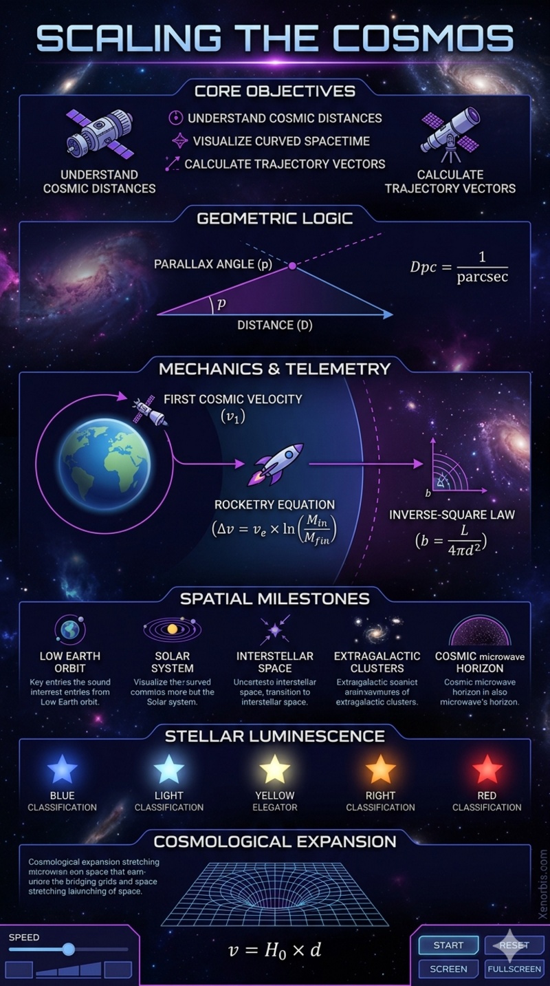
Modern astrophysics relies heavily on three-dimensional modeling to make sense of telemetry gathered by deep-space observatories. This specific visual tool serves multiple critical functions for engineers, researchers, and digital creators who require a grounded understanding of cosmic distances. Instead of viewing static statistics, users manipulate time and velocity parameters to witness exactly how rapidly local environments dissolve into massive interstellar networks.
In practical aerospace engineering and orbital mechanics, three-dimensional simulations are vital for calculating trajectory vectors, signal propagation delays, and gravitational assist pathways. By scaling down these enormous parameters into a single web-based application, this platform demonstrates the continuous transition between completely different regimes of physics, starting from planetary gravitation and ending with the dark-energy-driven expansion of the global cosmos.
The Geometric Logic of Astronomical Distances
☀ To navigate a digital universe accurately, a rendering engine must manage a series of drastically different measurement frameworks. Within our immediate cosmic backyard, scientists deploy standard metrics or convert them into operational constants based on mean distances. The average distance between the center of our planet and the center of the sun serves as the foundational yardstick for internal stellar systems, known universally as the astronomical unit.
As the simulation leaves the boundaries of local stellar systems, the astronomical unit becomes too small to remain computationally practical. At this stage, astrometry transitions to light-years or parsecs. A light-year represents the total distance a single photon travels through a perfect vacuum during one standard Julian year. When tracking the positions of remote stellar groupings, astronomers use the parsec, which represents the distance at which an object possesses a parallax angle of exactly one arcsecond. The mathematical translation between these spatial units follows strict geometric proportions:
Dpc = 1 / parcsec
Where Dpc represents the absolute distance measured in parsecs and parcsec denotes the observed parallax shift in arcseconds. Managing these shifts smoothly inside a rendering canvas requires dynamic camera adjustments to prevent visual clipping while maintaining crisp structural fidelity.
The Mechanics of Orbital Velocity and Flight Telemetry
Every celestial body inside this simulation behaves according to deep physical constraints. For an engineering module to maintain a stable trajectory around a primary planet without falling backward into the atmosphere, it must match or exceed the first cosmic velocity. This boundary represents the exact speed required to balance the inward pull of gravitational acceleration against the outward centrifugal tendency of a circular orbit.
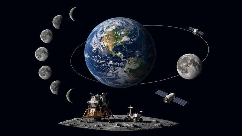
When the simulation transitions out of a localized path and initiates deep interstellar flight, the rendering framework scales up the environmental velocity. Real cosmic probes must calculate precise energy expenditures using foundational rocketry equations. The total change in velocity required to break free from a primary gravity well depends on the exhaust velocity of the propulsion engine and the precise mass ratio of the vessel before and after fuel consumption:
Δv = ve × ln(Minitial / Mfinal)
In this classic mathematical framework, Δv represents the net velocity adjustment, ve signifies the effective linear exhaust velocity of the engine, Minitial indicates the total starting mass including propellant, and Mfinal represents the dry structural mass of the craft. The speed slider on the control panel directly simulates these massive velocity shifts, transitioning the viewpoint across different scales of space-time metrics.
Spatial Milestones Across the Observable Universe
The architecture of the universe is highly clustered, consisting of massive hubs of matter separated by completely dark, empty voids. The table below details the core structural zones encountered during the simulation sequence, showcasing the primary physical constants and characteristic scales for each phase of flight.
| Simulation Stage | Standard Domain Scale | Dominant Physical Phenomenon |
|---|---|---|
| Low Earth Orbit | 200 to 2000 kilometers | Planetary gravity, atmospheric friction, and orbital centrifugal balance. |
| Solar System Interior | 0.1 to 50 astronomical units | Solar wind, Keplerian planetary motion, and radiation pressure. |
| Interstellar Space | 1 to 100,000 light-years | Stellar drift, molecular gas clouds, and galactic rotational curves. |
| Extragalactic Clusters | 1 to 100 megaparsecs | Gravitational binding of galaxy groups and dark matter scaffolding. |
| Cosmic Microwave Horizon | Greater than 45 billion light-years | Metric expansion of space-time and primordial relic radiation. |
The Mathematics of Stellar Luminescence
When rendering deep stellar backdrops, a computational model cannot simply display random points of light. True stars vary dramatically in color, surface temperature, and total energetic output. The absolute brightness of a star observed from a digital camera depends strictly on its intrinsic luminosity and its linear distance from the observation point. This relationship is calculated using the inverse-square law of light propagation:
b = L / (4 × π × d2)
Within this law, b represents the apparent brightness detected by an observer, L denotes the absolute intrinsic luminosity of the celestial source, and d represents the straight-line distance separating the observer from the star. As the camera pushes deeper into the cosmic void, nearby stars rapidly fade into the background, while massive stellar clusters merge into solid glowing structures, mimicking the optical limitations of real space telescopes.
🌟 Furthermore, the color of each individual star corresponds directly to its peak emission wavelength, which is determined by its surface temperature. Hot stars emit most of their radiation in the blue and ultraviolet spectrum, while cooler stars radiate primarily in the orange and red wavelengths, creating the vibrant visual diversity seen throughout the galactic flight phase.
Cosmological Expansion and the Deep Universe Boundary
At the ultimate limits of the simulation, the structural behavior of the cosmos undergoes a radical shift. Galaxies are not merely drifting through static space; instead, the very fabric of space-time is continuously stretching. This large-scale cosmological phenomenon causes remote objects to move away from an observer at speeds that scale proportionally with their distance. The foundational law governing this cosmic expansion is calculated by modern astrophysicists using a straightforward linear relationship:
v = H0 × d
Here, v signifies the apparent recessional velocity of a distant galaxy, H0 represents the current Hubble constant tracking the expansion rate of space-time, and d denotes the distance to the galaxy. Because of this continuous stretching, light traveling across immense cosmic distances is pulled into longer, redder wavelengths. This cosmological redshift sets an absolute physical boundary for what can be observed, transforming energetic ultraviolet rays into faint microwave signals by the time they reach our detection systems.
Metrics of Notable Cosmic Objects and Structures
To ground the virtual canvas in real physical telemetry, the rendering parameters utilize empirical data derived from centuries of observation. The table below displays the key physical statistics of confirmed cosmic structures that define our current understanding of the observable universe.
| Structure Designation | Estimated Physical Diameter | Approximate Total Mass Index |
|---|---|---|
| Planet Earth | 12,742 kilometers | 1.0 Earth Mass Unit |
| The Solar System | 150 billion kilometers | 1.0014 Solar Mass Units |
| Milky Way Galaxy | 100,000 light-years | 1.5 trillion Solar Masses |
| Virgo Supercluster | 110 million light-years | 1.2 quadrillion Solar Masses |
Normalized Engine Configurations for Web Graphics
To ensure high performance across multiple hardware devices, the simulation maps real-world physics onto a tightly optimized set of web constants. The table below defines the core parameters built into the JavaScript engine to balance mathematical accuracy with smooth interactive frame rates.
| Engine Identifier | Internal Value | Operational Target |
|---|---|---|
| Total Flight Frame Time | 180.0 seconds | Defines the temporal duration required to transit from Earth to the deep cosmic boundary. |
| Local Star Vector Count | 3000 points | Controls the density of nearby stellar coordinates without overloading gpu memory. |
| Galaxy Particle Count | 8000 points | Determines the structural resolution of the synthetic spiral galactic arms. |
The Role of Direct Screen Capture and Fullscreen Telemetry
A major feature of this engineering tool is the ability to extract crisp visual data directly from the active rendering buffer. By utilizing a preserved drawing matrix, users can freeze the current spatial configuration and download a pristine image file. This function is highly useful for generating educational assets, designing technical presentations, or analyzing specific geometric layouts of galactic structures.

When entering the fullscreen mode, the application automatically scales its viewport matrix to match the exact resolution of the output display. To prevent interactive overlays from distracting from the spatial view, the system triggers an automated visibility countdown. Moving the mouse or touching the screen instantly restores the telemetry inputs, giving users total control over their flight parameters while preserving unhindered visibility during long simulation flights.
Recommended Scientific Literature for Deep Spatial Study
- An Introduction to Modern Astrophysics — Written by Bradley W. Carroll and Dale A. Ostlie. Universally known as the definitive guide for understanding planetary mechanics, stellar evolution, and structural galactic dynamics.
- Foundations of Modern Cosmology — Written by John F. Hawley and Katherine A. Holcomb. An excellent scientific reference detailing the historic development and modern mathematics behind cosmic expansion models.
- Cosmology — Written by Steven Weinberg. A deeply rigorous mathematical text focused on the early universe, anisotropy constants, and general relativity applications on large cosmic scales.
- Stellar Structure and Evolution — Written by Rudolf Kippenhahn, Alfred Weigert, and Achim Weiss. This publication provides the core thermodynamic formulas used to calculate star brightness, mass indexes, and color spectrum outputs.

Julian D. Thorne — Celestial Mechanics Developer
Researcher and 3D engine developer focused on interactive stellar systems. Julian bridges the gap between theoretical physics and real-time browser-based cosmos exploration.


